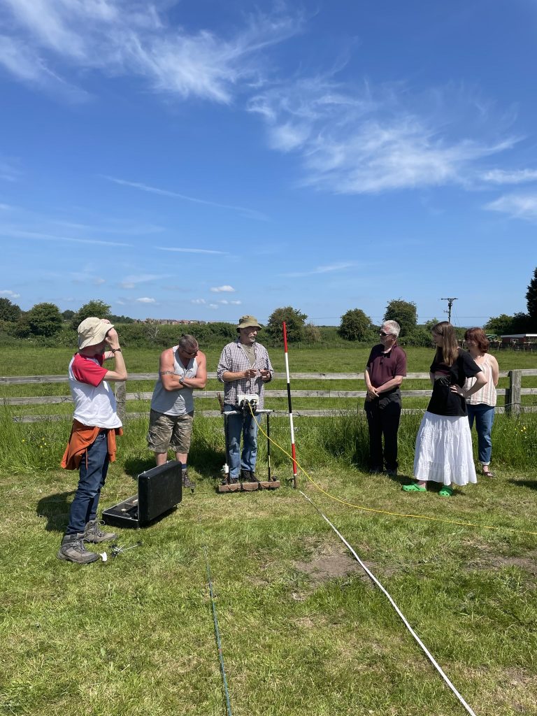
On a sunny Saturday in June, several of the GHAS committee took part in a geophysics survey in Kirk Hammerton. There was an amazing turn out for this community archaeology day, with 60 members of the local community taking part. I think the fantastic weather really helped as well!
The site in question is a investigation into a possible Neolithic henge at Kirk Hammerton, which Tony Hunt from YAA mapping has discovered. This has had quite a bit of publicity locally, and is really exciting find. Tony, along with community archaeologist Jon Kenny, did an excellent talk a couple of months ago for our friends at Kirk Hammerton History Society.
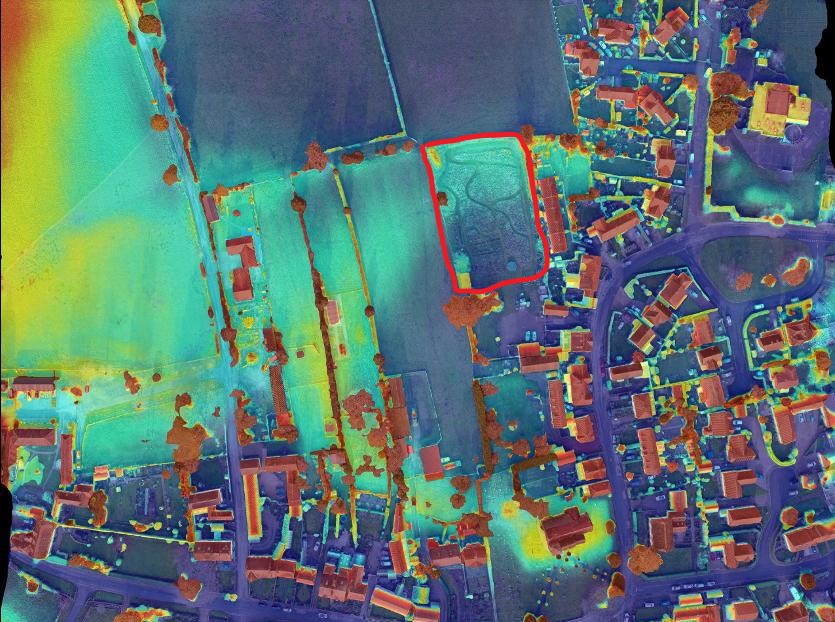
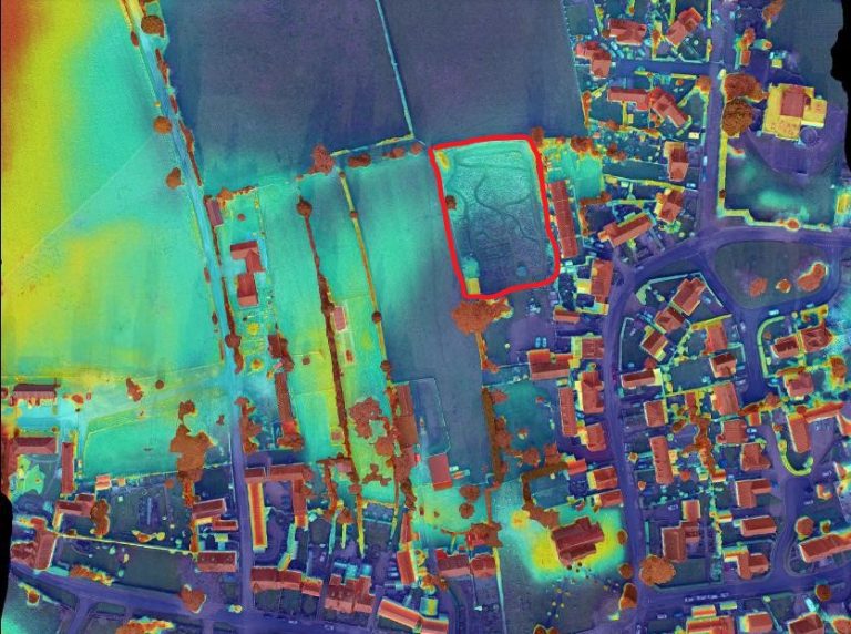
The red ring above is the field that we were surveying, and you can clearly see the ring of the henge from this aerial photo. Similar Neolithic henges across the region are around 200m across, and consist of a bank and ditch. The dimensions of the KH henge match this well. It’s also close to the River Nidd, and proximity to water is a common feature across many henges in this part of Yorkshire (for example at Thornborough).

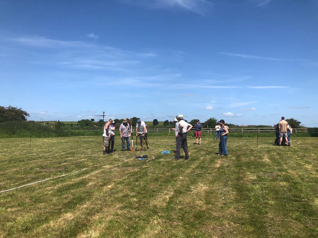
Under the guidance of Jon Kenny the geophysics survey was conducted over 3 20mx20m squares using a electrical resistance surveying.
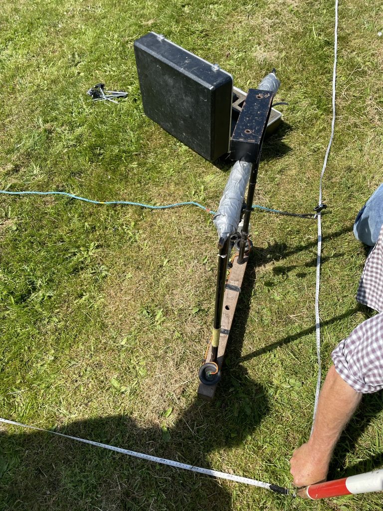
The electrical resistance survey works by passing a current through the ground from the two probes on the frame (in the picture above), to two other probes in the ground some distance away. A meter on the top of the frame measures the resistance through the ground, and what we are looking for are changes in the electrical resistance. This indicates a change in the nature of the ground, and can indicate a buried feature. For example, a stone feature might exhibit higher resistance, or a ditch (or what would have been a ditch) might show lower resistance.
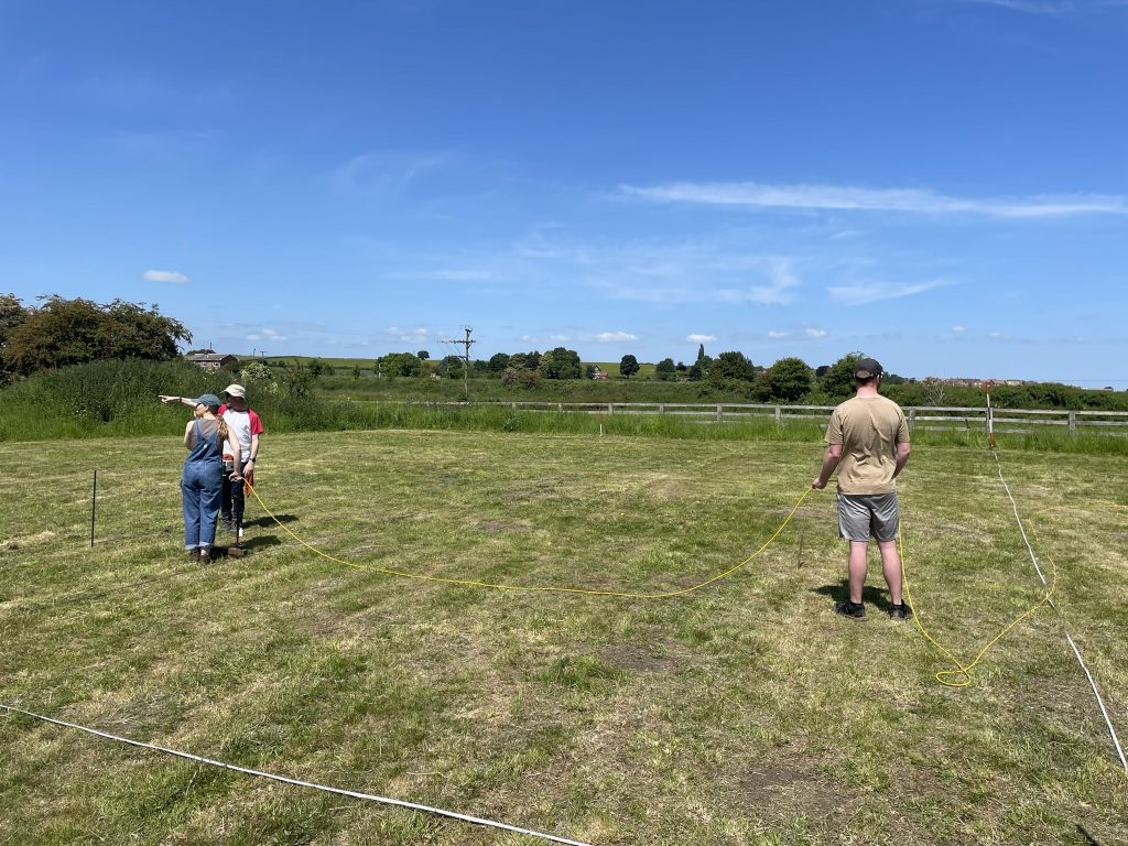
Once the grid is laid out and measured, and the machine setup, it is a simple case of working up and down the square, taking readings every 0.5m. This is done by inserting the probes on the frame into the ground.
The probes go into the ground, the logger beeps, and you move to the next point 0.5m further on. Working down the length of the square, we get 40 readings, then we work back down the square for the next meter. So in the end, each square has 40 x 20 readings. This process is then repeated for the next square and so on.
Once the data has been gathered, it can be fed into analysis software to see the results. Jon is going to do that as the next step, and we await the results with baited breath!